Inside a neural network

In the previous parts of this guide, we established a few important ideas:

1. A neural network is just a function. A complicated one, yes. But still a function. It takes numbers in and produces numbers out.
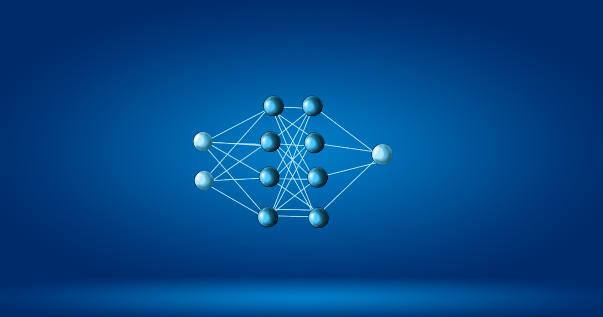
2. We also saw that neural networks follow a layered architecture. Instead of making one big leap from input to output, they move in small steps:
   1. The input layer receives raw numbers.
   2. Hidden layers transform those numbers step by step.
   3. The output layer produces the final prediction.
   4. For our running example, handwritten digits, the input is 784 pixel values. The output is 10 numbers, one for each digit 0 to 9. So the network’s job is clear.
3. Early layers apply very simple transformations. Later layers take those simple transformations and compose them into more meaningful ones. Layer by layer, raw data becomes more meaningful and easier to reason about.

What exactly happens inside a layer, though? What is the “transformation” the layer applies? To answer that, we need to zoom in, all the way down to a single neuron.

What does a neuron actually do?

A neuron does not “know” what an edge or a curve is. A neuron applies a rule to the numbers (inputs) it receives. That rule has three steps that translate to the following, in plain English:

1. Combine the inputs.
2. Add a small adjustment.
3. Decide how strongly to respond or fire.

When we say a neuron responds, we simply mean this: it produces a number. Think of this as the neuron asking itself: “How high or low should my output be?”

• A small number means: “The pattern I care about is probably not present.”
• A large number means: “The pattern I care about might be present.”

If that number is negative or close to zero, the neuron stays quiet and does not pass a lot of information forward. If the number is larger, the neuron passes a signal to the next layer.

That is all “firing” really means: a numerical signal strong enough to influence what happens next. Everything a neural network does is built from this simple operation, repeated thousands or millions of times.

Now let’s make this real.

How does this rule work in a realistic scenario, though? To understand this, let’s revisit our running example. I will peel this layer by layer. Please, run with me for a moment.

Zooming in on a single neuron

We are recognising a handwritten digit with 784 input neurons, each holding one pixel value scaled between 0 and 1. Imagine one neuron sitting in the first hidden layer of the network. This neuron receives all 784 pixel values from the input layer.

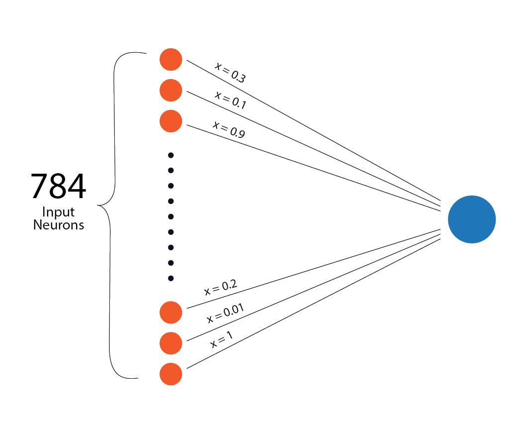
The neuron does not treat all inputs equally. Some inputs matter more, some matter less.

This is where weights come in.

Weights: how much each input matters

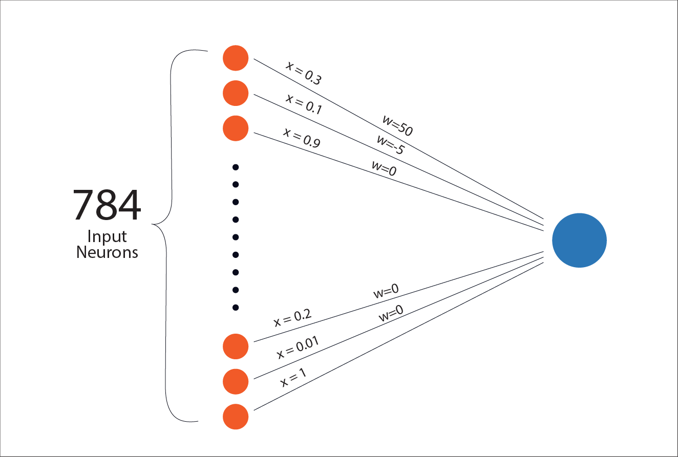
A weight is just a number that tells the neuron how important a particular input is. You can think of a neuron as asking: “How much should this input influence my final score?“

If a weight is large and positive, that input strongly pushes the neuron’s score upward. If it is large and negative, that input pushes the score downward. If it is close to zero, the input barely matters.

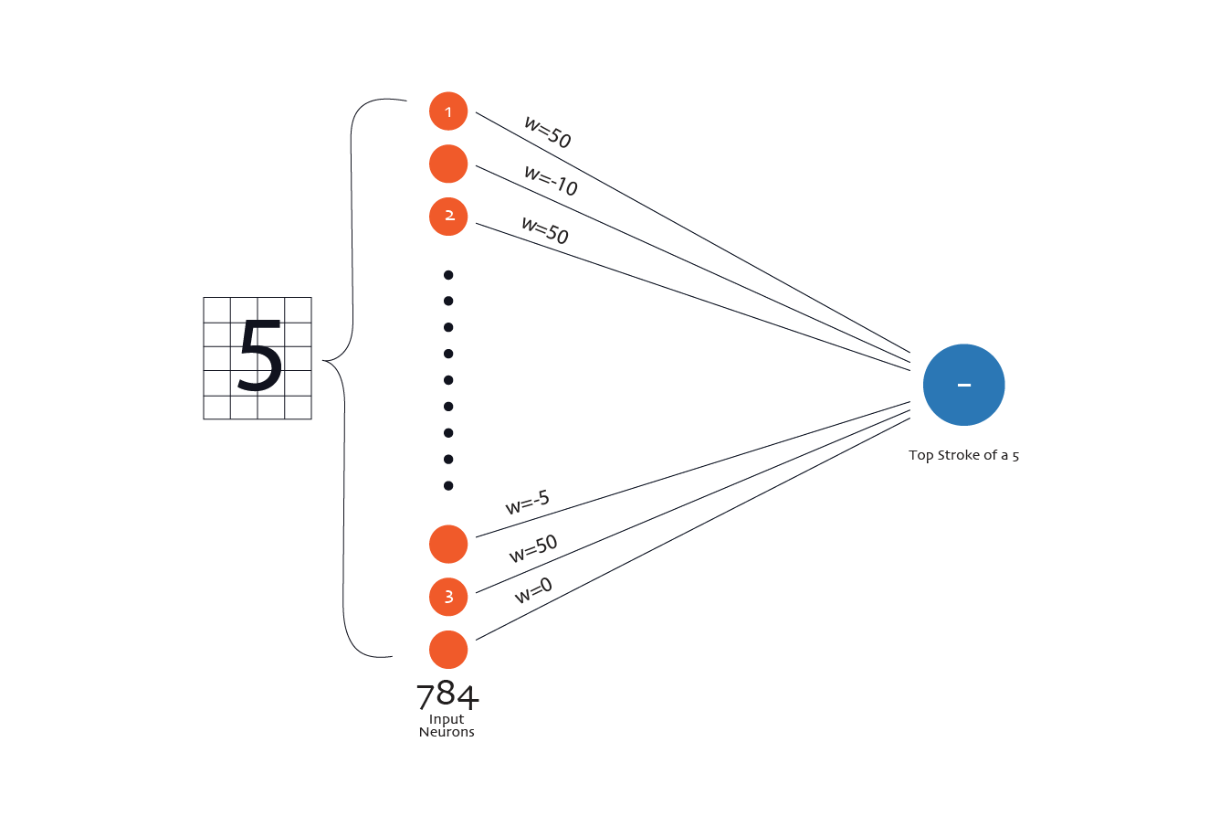
Let’s make this concrete with one specific neuron in the first hidden layer. Imagine this neuron eventually becomes useful for detecting the top horizontal stroke of a handwritten 5. Remember: this neuron receives all 784 pixel values as input. But only some pixels are relevant to that top stroke.

• Pixels that sit along the top row of the image, where the top stroke of a 5 usually appears, are important for this neuron.
• Pixels far from that region, say in the bottom-right corner of the image, are usually irrelevant for detecting a top stroke.

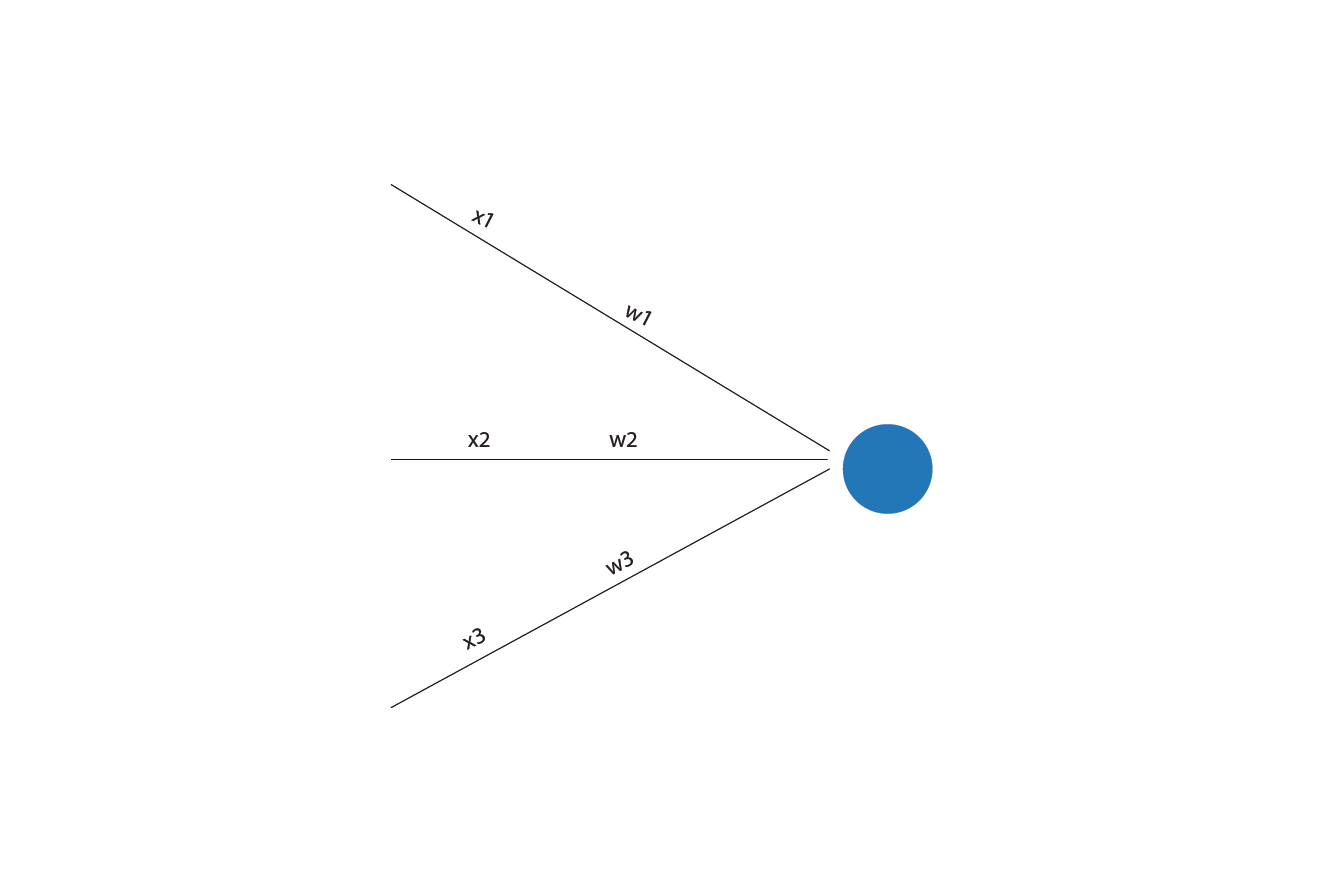
For demonstration, assume the relevant neurons are labelled 1, 2, 3 in the illustration below:

During training, the network adjusts the weights so that:

• The relevant neurons(1, 2, 3) that often light up when a top stroke is present get larger positive weights.
• Pixels that should usually be blank for a top stroke get negative weights.
• Pixels that do not reliably matter either way get weights close to zero. They barely influence the neuron.

So when an image of a handwritten 5 comes in:

• If the pixels along the top row are dark, the respective neurons in the input layer light up. Their large positive weights push the neuron’s output upward.
• If pixels that should be blank are dark, their negative weights push the output downward.
• If irrelevant pixels change, nothing much happens.

The neuron does not “know” it is looking for a top stroke. It simply produces strong output when the right combination of pixel values appears together. This is how neurons become sensitive to patterns. Not because we label patterns. But because weights make certain inputs matter more than others.

Mathematically, the neuron combines inputs like this:

weightedsum = (w₁ × x₁) + (w₂ × x₂) + ... + (wₙ × xₙ)

Where:

• x are the inputs.
• w are the weights.

Now, let's switch contexts for a second.

Weights: A non-technical view

Suppose you are deciding whether to attend a party and your decision depends on three factors:

• x₁: How close the party is.
• x₂: How tired you are.
• x₃: How much you like the people attending.

You do not weigh these equally.

• Distance might matter a little.
• Tiredness might matter a lot.
• Friends might matter even more.

Each factor pushes your decision in one direction or the other, with different strengths. Those “strengths” are weights. You might mentally combine them like this:

• A nearby party nudges you toward going.
• Being very tired pulls you strongly toward staying home.
• Close friends pull you back toward going.

You do not consciously multiply numbers. But you are doing something similar. You are combining signals. Each signal has a different importance. You end up with one internal score: “Do I go or not?”

A neuron does the same thing, but more literally.

• Each input number is multiplied by its weight.
• All those weighted inputs are summed.
• The result is a single score that reflects how strong the overall evidence is.

If the evidence points strongly in one direction, the neuron responds strongly. If the evidence is weak or conflicting, the neuron barely responds.

So when we say “this neuron cares more about certain inputs”, we mean something very literal: Those inputs have larger weights, so they contribute more to the neuron’s final score.

A neuron as a chef

Here is a helpful way to hold the whole picture in your head. Think of a neuron as a chef in a restaurant.

• Ingredients come in. These are the inputs.
• The chef mixes them in specific quantities. These are the weights.
• Then the chef adds a personal touch. That is the bias.

Two chefs can receive the same ingredients but produce different meals. Because they use different quantities and different personal touch. That is exactly what is happening in a neural network.

• Each neuron receives numbers.
• Each neuron mixes them differently.
• Each neuron produces its own output score.

Now let’s talk about that “personal touch”.

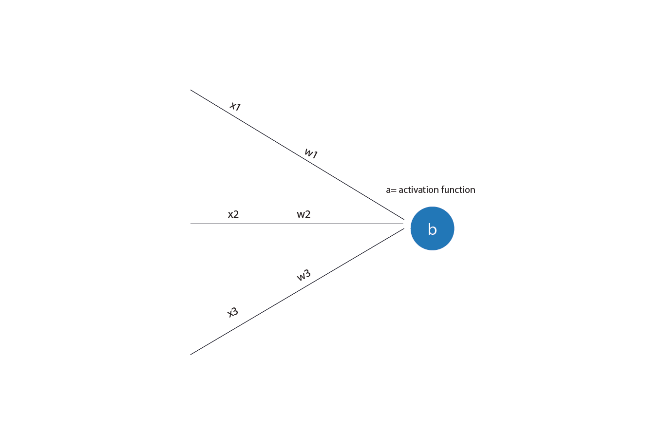
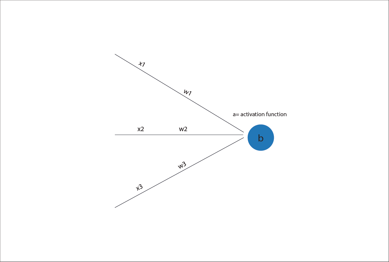
Bias: the baseline tendency

There is one more piece before the neuron makes a decision: the bias.

The bias is a built-in offset. It controls how easily or how hard a neuron responds. When a neuron responds strongly enough to pass a meaningful signal forward, we say the neuron activates (or fires). These two words mean the same thing, and from this point on, we will mostly use the term activation.

Even before looking at the inputs, the neuron starts with a small push toward either activation or silence. A positive bias makes activation easier. The neuron needs less evidence from its inputs to activate. A negative bias makes activation harder. The inputs must collectively be stronger before the neuron responds.

In simple terms, the bias sets the neuron’s default tendency. It decides whether the neuron is eager to activate or cautious, even before any inputs are considered.

The bias is usually added to the weighted sum. Mathematically, the neuron computes:

z = (w₁ × x₁) + (w₂ × x₂) + ... + (wₙ × xₙ) + b

Where b is the bias.

But why is the bias needed? Because sometimes, even if all inputs are zero or small, you still want the neuron to have a baseline tendency to activate.

Back to the party example. Even if the party is not close, you are somewhat tired, and the guest list is unknown, you might still go. Because you are generally social. That “default tendency” is the bias. In other words, some people are naturally social. Even with weak reasons, they lean toward going. Others need strong reasons to say yes. That baseline inclination is the bias.

Your final decision comes from combining the factors, weighting them, adding your baseline tendency, and seeing where you land. A neuron does the same thing, just with numbers.

Connecting this back to handwritten digits

In a fully connected neural network:

• Every neuron in a layer connects to every neuron in the previous layer.
• Every connection has a weight.
• Every neuron has its own bias.

So:

• Each neuron in hidden layer 1 has 784 inputs (x) and weights (w), one for each input pixel.
• Each neuron in hidden layer 2 receives an input from every neuron in hidden layer 1 and has weights for each input.
• Each output neuron has weights for every neuron in the last hidden layer.

So when we say “This neuron detects a vertical stroke,” what we really mean is that this neuron has learned weights and a bias such that certain combinations of inputs, usually from neurons in the previous layer, push its output high. The neuron does not output a label “edges”. It responds to patterns of numbers that happen to correspond to edges.

Why our neuron description is still incomplete

Up to this point, we have described a neuron as doing three things:

1. Taking in numbers.
2. Combining them using weights and a bias.
3. Producing a score.

This description is correct. But it is still missing something important. So far, everything the neuron has done is linear. And linearity, on its own, is not enough to build powerful neural networks. To see why, we need to slow down and talk about what linear really means.

What linearity actually means

A linear rule is one where outputs change in direct proportion to inputs. If you double the input, you double the output. If you add two inputs together, their effects simply add. A straight line is the perfect visual example of a linear relationship.

For instance:

• If exam scores increase, the chance of passing increases.
• If house size increases, price increases.
• If brightness increases, pixel value increases.

Linear rules are simple, predictable, and easy to understand. Traditional models such as linear and logistic regression rely on linear combinations of features. And for many problems, this works well. But linear rules have a hard limit.

No matter how many linear operations you stack together, the result is still linear. A straight line composed of another straight line is still a straight line. Mathematically, this means: A stack of linear layers can always be collapsed into a single linear layer. This is the key problem.

Why linearity is not enough for neural networks

Real-world problems are rarely linear. Consider handwritten digits. There is no single straight boundary that separates all images of “5” from all images of “3” or “8” in the space of 784 pixel values. The relationship between pixels and digits is tangled, curved, and full of exceptions.

If every layer in a neural network were linear, then no matter how many layers we added, the network would still behave like a single-layer model. It would not gain expressive power. It would fail at exactly the same kinds of problems.

So if linearity is not enough, what is?

Nonlinearity!

To model complex patterns, we need non-linear transformations. Non-linearity allows:

• Small input changes have different effects in different regions.
• Multiple simple patterns to combine into richer ones.
• Curved, folded, and irregular decision boundaries.

In plain terms, nonlinearity allows the network to bend space rather than draw straight lines through it. This is what enables neural networks to handle messy problems such as handwriting, speech, language, and images.

But how does a neural network introduce non-linearity? This is where activation functions come in.

Activation functions: introducing nonlinearity

An activation function is a rule applied after the neuron computes its weighted sum. Instead of passing the raw score forward, the neuron passes the score through a non-linear function. So the neuron’s computation becomes:

weighted_sum = (w₁ × x₁) + (w₂ × x₂) + ... + (wₙ × xₙ) + b
output = non_linear_activation_function( weighted_sumz)

Note: the intermediate weighted_sum is often written z

This small change makes a huge difference. The weighted sum on its own is linear. The activation function breaks that linearity. By stacking layers of neurons that include activation functions, neural networks gain the ability to model complex, non-linear relationships.

Before we go further, it is worth noting that there are many activation functions. Over the years, researchers have proposed dozens of them. Some were popular in the early days of neural networks. Others are still used in specialised settings today. But for our purposes, and for most modern neural networks, we only need to focus on two.

Why? Because each part of the network has a different job.

• Hidden layers are about discovering useful internal patterns.
• The output layer is about making a clear, final choice.

That difference is why we use ReLU in the hidden layers and Softmax at the output.

ReLU

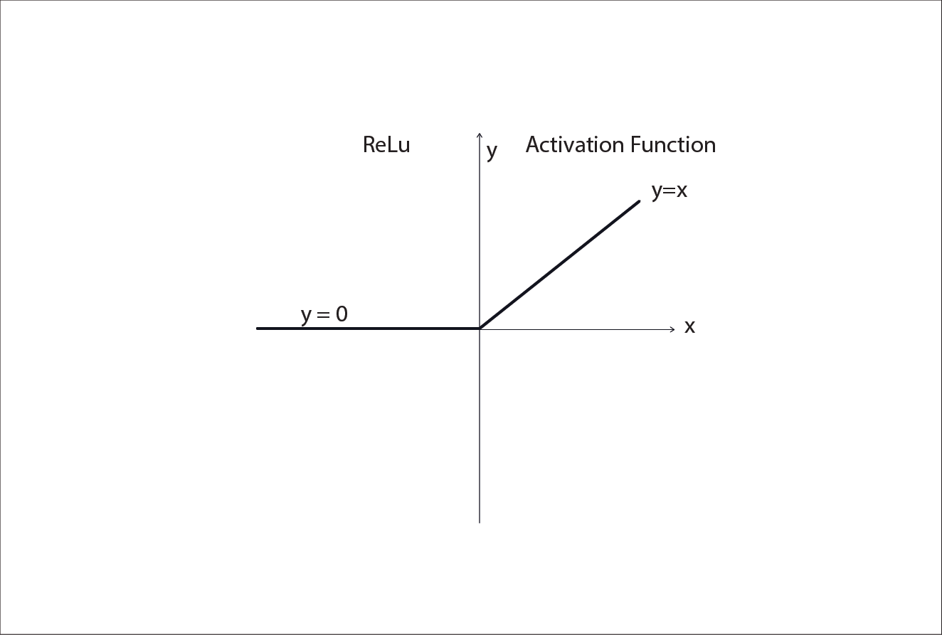
In modern neural networks, a widely used activation function for hidden layers is ReLU, short for Rectified Linear Unit.

It is defined as:

ReLU(z) =max(0, z)

In plain language:

• If the neuron’s raw score z is negative, the output is 0.
• If z is positive, the output is passed through unchanged.

This creates a very intuitive behaviour:

• Weak or irrelevant signals are shut off.
• Strong signals are allowed to flow forward.

Returning to our party analogy, if all considerations (distance to the party, which friends are going, weather, etc.) lead to a positive score, then you go. If, instead, they result in a negative score or zero, nothing happens; you stay at home regardless of how bad the combination of factors is.

ReLU is simple, fast to compute, and works remarkably well in practice. That is why it is the default choice for most hidden layers, including our handwritten digit recogniser.

What about the output layer? Enter Softmax

Remember, deep neural networks are made of several layers of neurons. The “intermediate layers” (from the inputs through the ones before the last) are called “hidden”. The output layer is the last set of neurons we look at to read the prediction.

Moving on, the hidden and output layers have different roles. Hidden layers build internal representations. The output layer must produce a final decision.

In our digit recognition example, the output layer produces 10 numbers, one for each digit from 0 to 9. We want these numbers to behave like probabilities. This is where the softmax activation function is used.

Softmax takes a list of numbers and:

• Converts them into values between 0 and 1.
• Ensures they all add up to 1: Having the scores of each possible output sum to 1 has nice properties. It allows humans to interpret the model's confidence and works well with loss functions during training. Nevertheless, you must keep in mind that while it's convenient to think of these outputs as probabilities, this interpretation is not entirely accurate unless the neural network has gone through some extra work (called calibration).

In effect, softmax answers the question: “Given all these possibilities, how confident am I in each one relative to the others?”

After softmax:

• A high value means high confidence.
• The largest value determines the network’s prediction.

This makes softmax ideal for multi-class classification tasks like digit recognition.

Putting it all together

With activation functions in place, a neuron now does the following:

1. Computes a weighted sum of its inputs.
2. Adds a bias.
3. Passes the result through a non-linear activation function.

This is the missing piece. So, for example, if the activation function is ReLU, mathematically, the

output = max(0, (Σ (wᵢ × xᵢ) + b ))

That output becomes an input to the next layer. This is the transformation we talked about earlier. Each layer applies many of these transformations in parallel. Layer by layer, the data is reshaped.

From pixels to prediction

With this rule in place, the network’s forward pass becomes clear. The image enters as 784 pixel values.

Hidden layer 1:

• Each neuron computes a weighted sum plus bias
• Applies ReLU
• Outputs a new set of numbers

Hidden layer 2:

• Repeat the same rule on those new numbers
• Outputs another set of numbers

Output layer:

• produces 10 numbers: one score per digit 0 to 9 (you will often see this called ‘logits’)
• Applies softmax activation
• Produces 10 probability-like scores (one per digit 0-9)
• The highest score becomes the prediction

That is the internal journey. Numbers in, numbers transformed, numbers transformed again and finally, decision out.

In other words, early layers learn weights that respond to simple patterns. Later layers combine those responses into richer representations. The output layer uses those representations to make a decision. Nothing is hand-coded. The network does not learn what to represent. It learns whatever representations help it perform the task.

What we have not explained yet

We now know what is inside a neuron. But the most important question is still waiting: Where do the weights and biases come from? How does the network know when it is wrong? How are weights adjusted during training?

Those questions lead us to the final missing piece: How a neural network learns.

Up next: How neural networks learn

In the next part, we will focus entirely on the learning process. We will see how a network makes a prediction, measures its error, sends that error backwards through the layers, and updates its weights and biases to improve.