In the previous part of this guide, we opened up the black box of a neural network and looked inside a single neuron. We saw that a neuron follows a very simple rule.

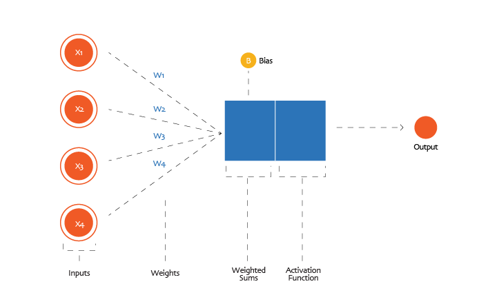
1. It receives numbers as inputs.
2. It multiplies each input by a weight.
3. It adds a bias.
4. It passes the result through an activation function.
5. It sends the output forward to the next layer.

Mathematically, a neuron computes something like this:

weighted_sum and bias = (w₁ × x₁) + (w₂ × x₂) + ... + (wₙ × xₙ) + b
output(activation) = non_linear_activation_function( weighted_sum)

This happens in every neuron, across many layers. Each layer transforms the numbers a little more, gradually turning raw pixel values into more meaningful signals, until the output layer produces a final prediction.

Underneath all of this are two key elements: weights and biases. These are the network’s internal parameters. When you hear that a model has 100 million parameters, these are often the types of parameters being referred to. They control how strongly each neuron responds to its inputs and therefore determine how the network behaves.

If the weights and biases are well chosen, the network performs well. If they are poorly chosen, the network performs terribly. This naturally raises the most important question in neural networks: How do we find the right weights and biases?

The central idea of learning

Up to this point, we have described how a neural network makes a prediction. But we have not yet explained how it learns to make good predictions. Who chooses the values of the weights? Who decides the biases?

Well, they are not handwritten by engineers. Engineers write code for the training process. Then, during training, the model gradually learns the weights and biases. When we say a neural network is training, we mean something very specific: The network is searching for the set of weights and biases that allows it to perform well on a given task; performing well means making only tiny errors. Learning is simply an optimisation process.

The network starts with random parameters and gradually adjusts them until its predictions become accurate. In this part of the guide and the next, we will unpack exactly how this happens.

We will take our time with this, starting from the very beginning.

Training a neural network: the big picture

Training is the process of guiding a neural network toward a good set of weights and biases.

Let us anchor the discussion in our running example: handwritten digit recognition. We want our neural network to look at a 28×28 black and white image and correctly classify the digit from 0 to 9.

• Consequently, our input layer would contain 784 neurons, one for each pixel.
• Our network could also have 2 hidden layers, each with 16 neurons. This is admittedly an arbitrary choice, but it keeps the example simple.
• Our output layer contains 10 neurons, one for each digit.

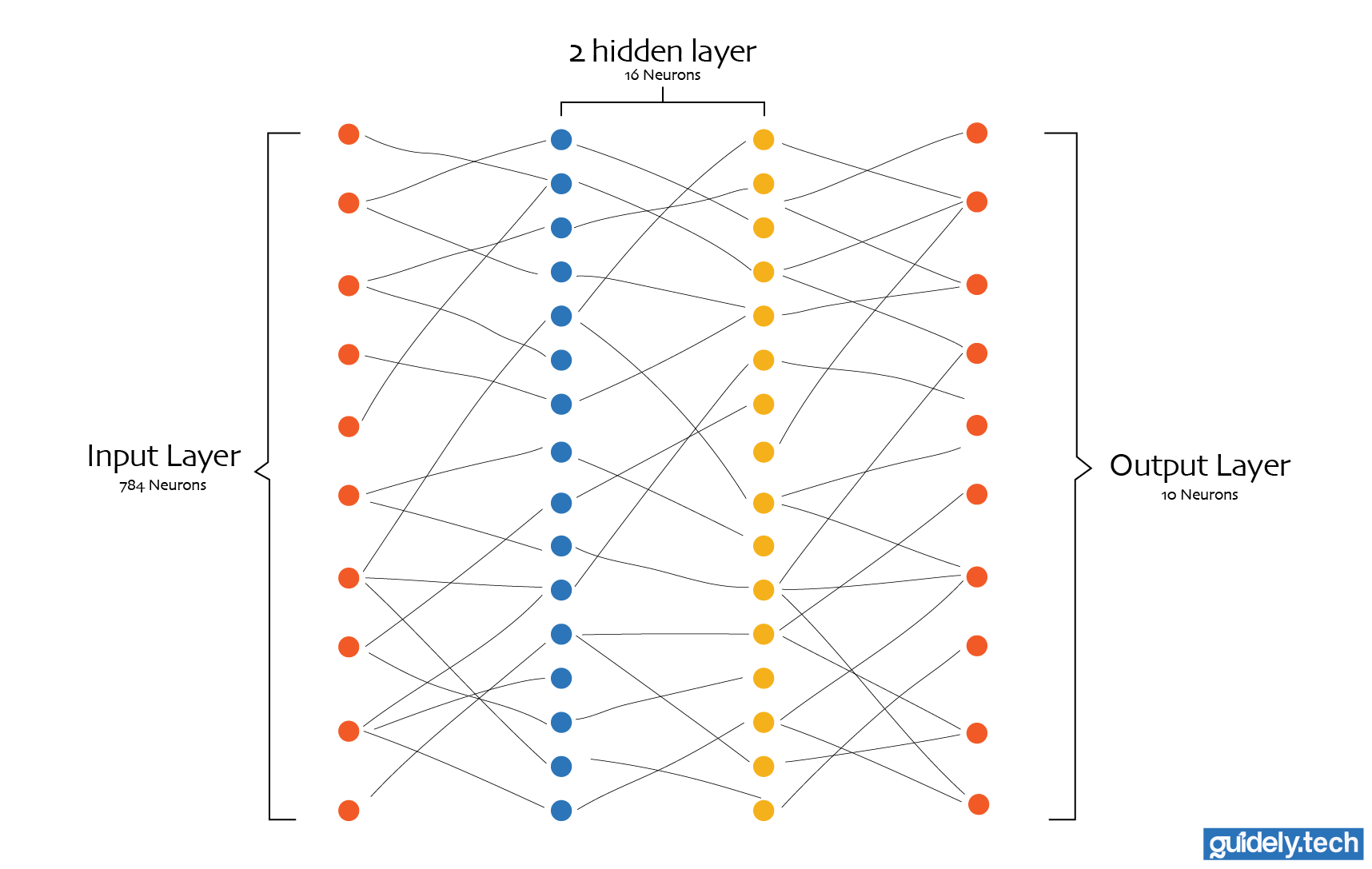
Even a network this small contains a surprising number of parameters. In a fully connected neural network, every input is connected to every neuron in the first layer, and each neuron in turn is connected to every neuron in the next layer, all the way to the output neurons. Each connection carries a weight, and every neuron (except the input neurons) has a bias.

When we account for all of these connections and biases across the network, this architecture contains:

• Between the input layer and the first hidden layer = 784*16 = 12,544 weights
• Between the first hidden layer and the second hidden layer = 16*16 = 256 weights
• Between the second hidden layer and the output layer = 16*10 = 160 weights

Total weights = 12,544+256+160 = 12,960

Each neuron has one bias. Therefore, the number of bias parameters is equal to the sum of neurons.

Total biases = 16 + 16 + 10 = 42

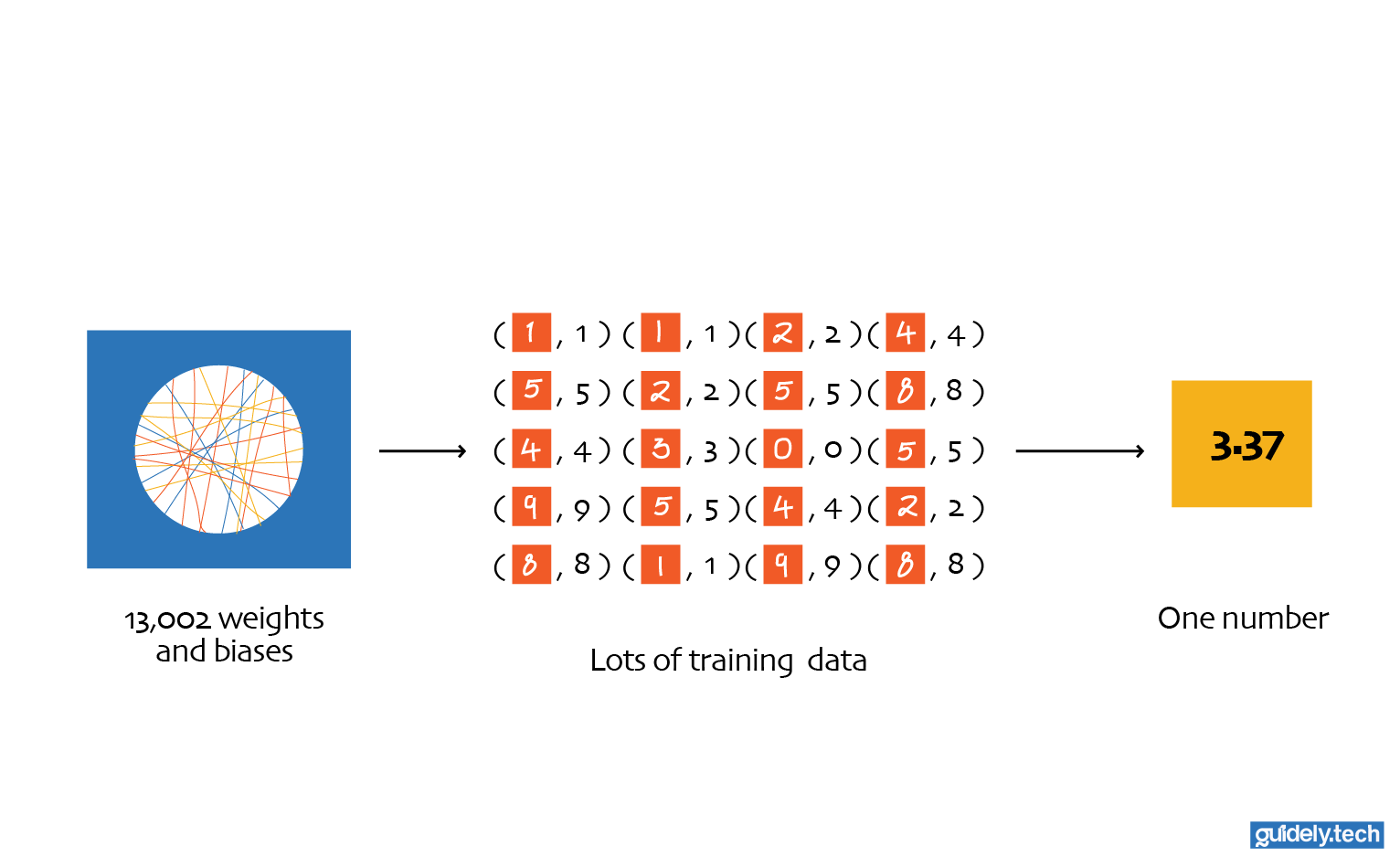
Total parameters = 12,960+42 = 13,002

Training this neural network means guiding it toward the right set of values for those 13,002 parameters. When the values are poor, the network produces poor predictions. When the values are good, the network becomes surprisingly accurate at recognising handwritten digits.

How do we “guide” this network toward the right set of weights and biases?

How a neural network learns

A quick refresher: In traditional software, engineers write explicit instructions for the computer to follow. If you wanted a program to recognise handwritten digits using traditional programming, you would have to carefully write rules for detecting strokes, curves, loops, and other patterns that define each digit.

Machine learning takes a very different approach. Instead of writing rules for recognising digits, we write an algorithm that learns the rules from examples. In our case, we provide the network with many images of handwritten digits along with the correct corresponding number. The training algorithm then adjusts the network’s 13,002 parameters until the network becomes good at recognising digits on its own.

In other words, we do not program the network to recognise digits. We program it to learn how to recognise digits.

Training data and test data

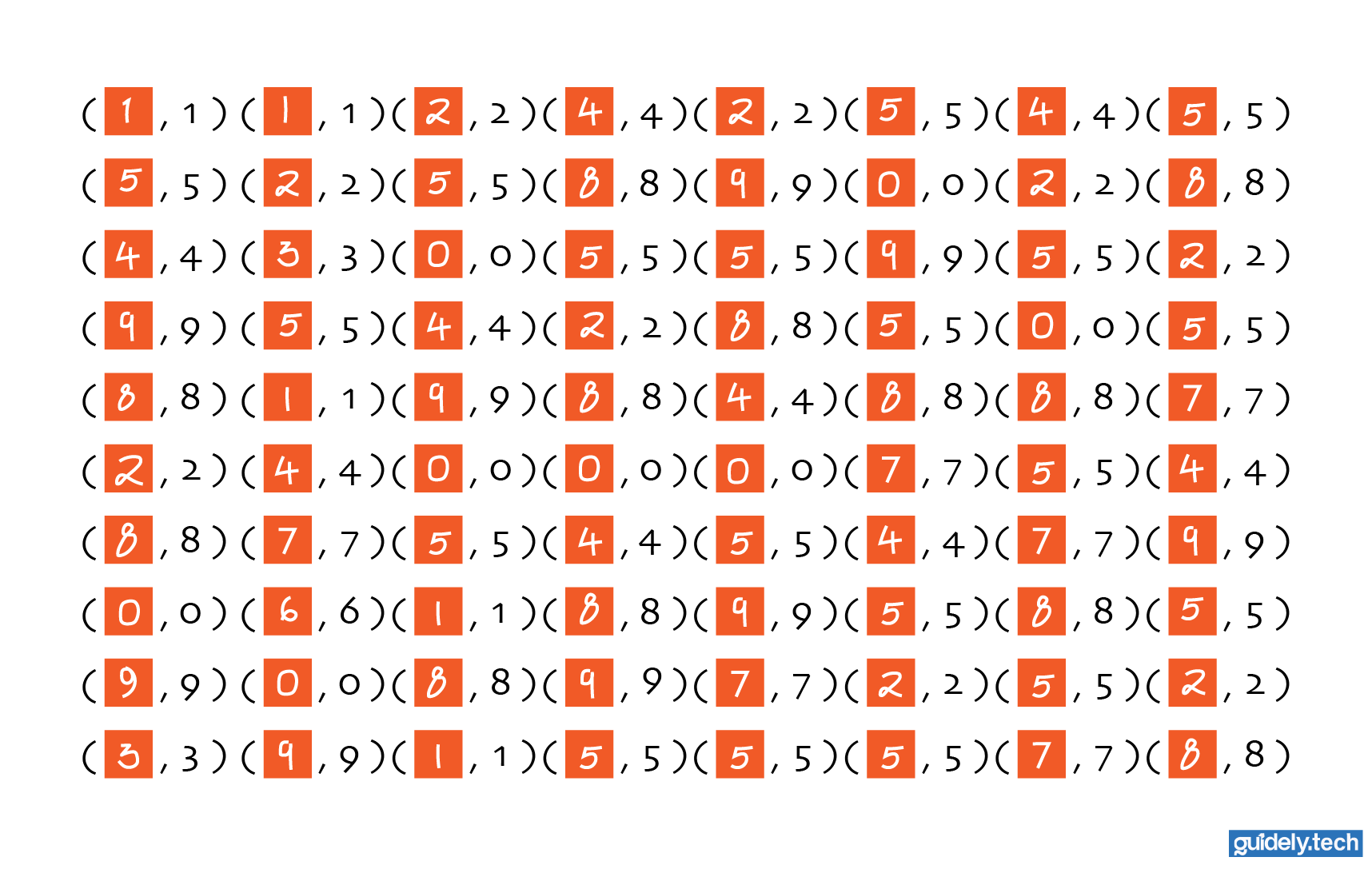
The examples we feed into the network are called the training data. Each example in the training data contains two things:

• An input image (the 784 pixel values)
• The correct label (which digit the image represents)

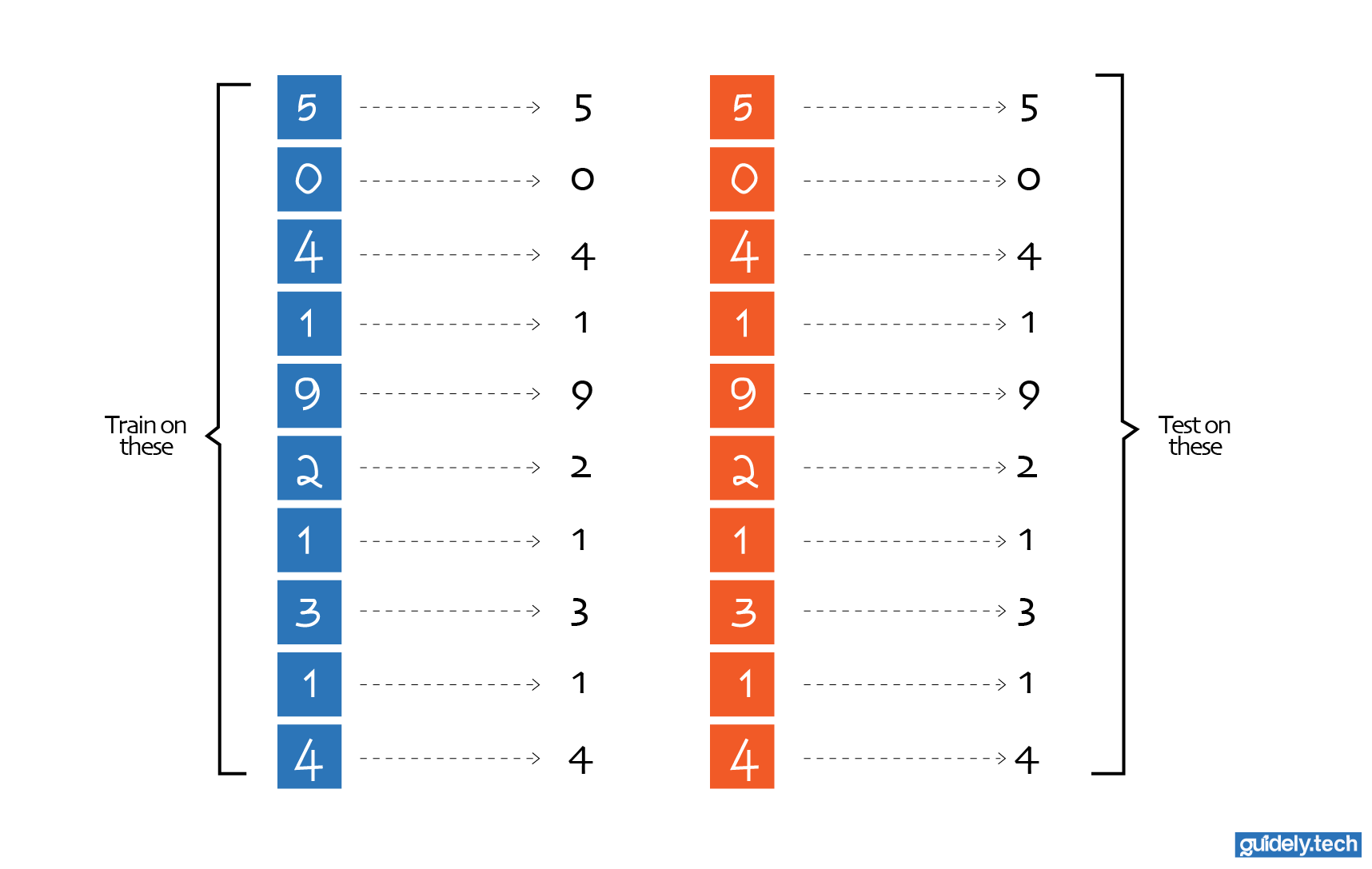
By repeatedly looking at these examples, the network gradually learns patterns that help it distinguish between digits. However, we also want to know whether the network has truly understood the task or simply memorised the training data.

To evaluate the network, we first shuffle the data and then split it into two. The larger part (for example, 90%) is used for model training, while a smaller part (e.g. 10%) is reserved and used only afterwards to verify that it has truly learned the task. If so, the neural network should be able to generalise and correctly identify the digit in those reserved test images. The smaller part, the 10%, is called the test data. If the network performs well on both the training data and the test data, it suggests that the patterns it learned generalise to new images.

Fortunately, we do not have to collect these examples ourselves. Researchers have already assembled a widely used dataset for this task called the MNIST database. MNIST contains 70,000 images of handwritten digits, each labelled with the correct number. This dataset has become a standard benchmark for training and evaluating digit recognition systems.

What training actually looks like

With the dataset in place, we can begin the training process. Training starts by initialising all the weights and biases in the network with random values. At this point, the network has no understanding of digits. Its predictions are essentially random guesses.

From there, training follows a simple loop:

1. Feed the network an image from the training data.
2. Let the network produce a prediction.
3. Compare the prediction with the correct label.
4. Measure how wrong the prediction is.
5. Adjust the weights and biases slightly to reduce that error.

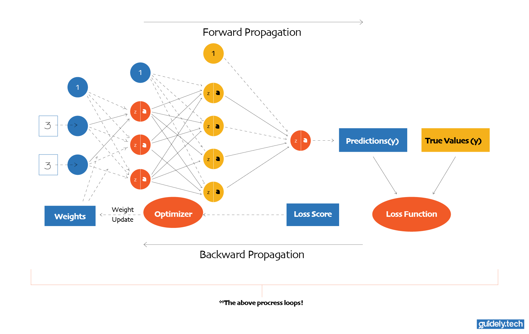
Then we repeat the process. This loop runs thousands or millions of times. With each step, the network’s parameters shift slightly toward values that produce better predictions. Over time, the network gradually improves. What begins as random guessing slowly turns into reliable digit recognition. This process is what we mean by neural network learning. But two crucial questions remain:

• How exactly do we measure how wrong a prediction is?
• And once we know that, how do we determine how the weights and biases should change?

To answer these questions, we need three key ideas:

• Loss function
• Gradient descent
• Backpropagation

In this part of the guide, we will explore the first two.

Measuring error: the loss function

To improve the network, we first need a way to measure how wrong it is. This is the role of the loss function. A loss function takes the network’s prediction and the correct answer and returns a number representing the error for a single example.

• Large error → high loss → The network’s prediction is far from the correct answer
• Small error → small loss → The network’s prediction is close to the correct answer

You can think of the loss function as a wrapper around the neural network. The neural network itself is a function:

prediction = neural_network(input, weights, biases)

The cost function builds on top of this:

loss = loss_function(prediction, correct_label)

Now here is the important connection.

The prediction itself depends on the weights and biases. If we change the weights and biases, the prediction changes. And if the prediction changes, the loss changes. So even though the loss function appears to take only a prediction and a label, it is directly tied to the network’s parameters.

If we combine both expressions into one, we get:

loss = L(neural_network(input, weights, biases), correct_label)

Mathematically, for a single training example:

Where:

• $f(x; w, b)$ is the prediction of the network on an example image $x$
• $L(\cdot)$ is the loss function
• $w, b$ are the weights and biases
• $y$ is the corresponding correct number for the input image $x$

So when we say, “The loss tells us how good the network is,” what we really mean is: “The loss tells us how good the current weights and biases are for this example.”

This is why the loss function is so important. It gives us a single number that depends on all the network's parameters. By trying to reduce this number, we are indirectly guiding the network toward better weights and biases.

A concrete example

Suppose the network receives an image of the digit 3. After passing through the network, the output layer produces ten numbers:

[0.02, 0.01, 0.10, 0.90, 0.03, 0.02, 0.04, 0.03, 0.03, 0.02]

Each number corresponds to a digit from 0 to 9, in order.

• So the position of each number in the output vector indicates which digit it represents. Now, looking at the output: The largest value is 0.90, and it appears in the fourth position. Since we start counting from 0, the fourth position corresponds to the digit 3.

So the position of each number in the output vector tells us which digit it refers to. Now, looking at the output: The largest value is 0.90, and it appears in the fourth position. Since we start counting from 0, the fourth position corresponds to the digit 3.

In this case, the prediction is correct.

But what does “correct” actually mean numerically? For this input, the ideal output is a vector where the correct digit has a value of 1, and all others are 0:

[0, 0, 0, 1, 0, 0, 0, 0, 0, 0]

Now we can compare what the network produced with what we want. To measure how good the prediction is, we use a classification-specific loss function: categorical cross-entropy.

Where:

• $a_i$ is the predicted probability for class $i$, in our case 3
• $y_i$ is the true label (1 for the correct class, 0 otherwise)

Because only one $y_i$ is 1, this simplifies to:

For the correct prediction above, where the network assigns 0.90 to the correct class (digit 3), the loss is:

Using the natural logarithm base $e$

This is a relatively small value, indicating low loss and, by extension, good prediction.

Now imagine the network outputs:

[0.02, 0.01, 0.10, 0.20, 0.03, 0.45, 0.04, 0.03, 0.03, 0.09]

Here, the network believes the image is 5, because 0.45 is the largest value. While the correct class (digit 3) now has a probability of 0.20. Loss is:

This is much larger, indicating high loss and, by extension, poor prediction.

This is the key idea: The loss function does not just check if the prediction is right or wrong. It measures how confident the network is in the correct answer.

• If the network is correct and confident → loss is low
• If the network is wrong or uncertain → loss is high

This single number gives us a clear signal of how good or bad the current weights and biases are for that example.

Cost across an entire dataset

In practice, we do not evaluate performance using just one example. We evaluate it across many examples. Each example produces its own loss. We then average these losses to get the cost function: In our case, the MNIST dataset contains 70,000 examples, let’s represent that number with m. We compute the cost for each example and then average them:

Where:

• $m$ is the number of training examples
• $L$ is the loss for a single example
• $\hat{y}$ is the prediction

This average tells us how well the current weights and biases perform across the dataset. Our goal is simple: Find the set of weights and biases that produces the lowest possible cost. This means finding the minimum of the cost function.

How do we compute this minimum?

Finding the minimum of the cost function: the landscape analogy

You can imagine the cost function as defining a landscape. Every possible combination of weights and biases is a point in this landscape. The height of that point is the cost.

• High points mean high cost. These correspond to bad parameters, where the network makes poor predictions.
• Low points mean low cost. These correspond to good parameters, where the network performs well.

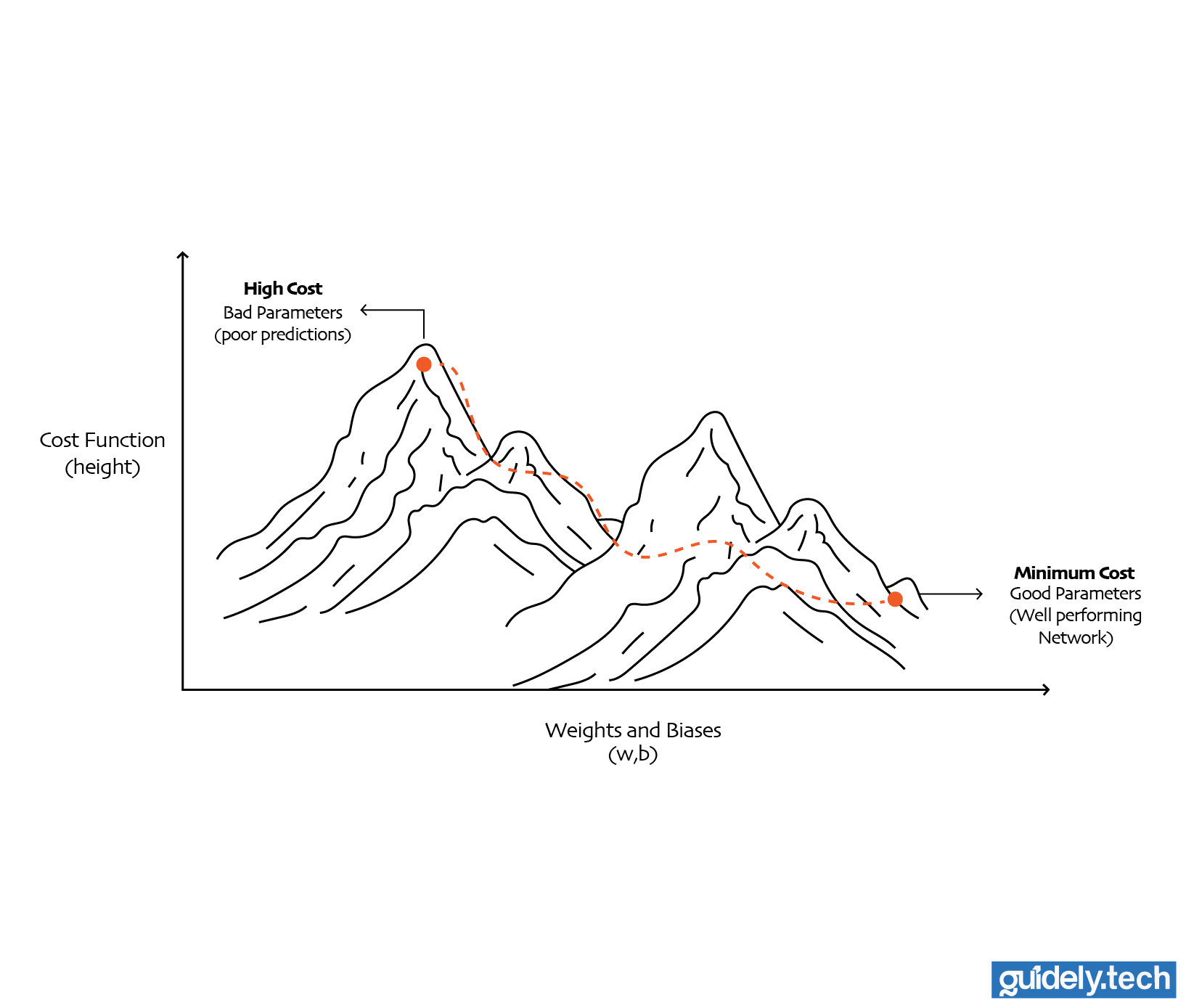
So the goal of training becomes very clear: We want to move through this landscape and find the lowest point, the set of weights and biases that gives us the smallest possible cost. In our case, that means finding the best values for all 13,002 parameters so the network can accurately recognise handwritten digits.

But here is the problem.

Since our neural network has 13,002 parameters. The landscape, therefore, exists in a space with 13,002 dimensions. Evidently, this is not a simple 2D landscape, so how do we find the set of weights and biases that would minimise our cost function?

The simplest idea (but impractical)

The most straightforward idea would be brute force. We could try many random combinations of weights and biases and keep the best ones. But remember, we are dealing with a space of 13,002 dimensions. At that scale, trying out every possible combination of parameters is completely unrealistic.

So the real question becomes: How do we move through this high-dimensional landscape in a smart way, so that we reliably move toward lower cost, without checking every possible point?

This is where the idea of slope comes in.

Using the slope as a signal

At any point on the landscape, the slope tells us how steep the surface is and in which direction it rises. If we can measure the slope, we can use it as a signal to decide how to move.

Now, let us connect this intuition to mathematics.

In basic calculus, the derivative tells us the slope of a function, in other words, how the output changes when we nudge the input slightly.

• If the derivative is positive, increasing the input increases the output.
• If the derivative is negative, increasing the input decreases the output.

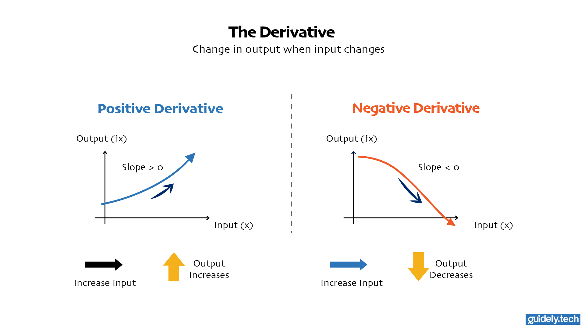
This simple idea turns out to be the key to improving a neural network.

For a moment, let us forget our digit recogniser with its 13,002 parameters. That is too much machinery at once. Instead, let us start with the smallest possible example and build up from there.

Imagine a very simple network with just one input and one parameter. It takes in a number x and produces an output:

Here, w is the only parameter. It controls how strongly the input affects the output.

Now, suppose this little network performs terribly at its task. The natural question is: how do we improve it? I need you to pause and think here a bit: With everything you know so far, what steps would you take to improve its performance?

Well, we already know the answer at a high level. We wrap the network in a cost function so we can measure how bad its current parameters are. Since the prediction depends on w, the cost also depends on w. So instead of just writing the network as f(x) = wx, we also think about a cost function like this:

This notation means: the cost is a function of the parameter w. Now comes the important step. We take the derivative of the cost with respect to w:

This derivative tells us how the cost changes if we nudge w slightly.

• If the derivative is positive, increasing w would increase the cost. That is bad, so to improve the network, we should decrease w.
• If the derivative is negative, increasing w would decrease the cost. That is good. To improve the network, we should increase w.

This is the core idea of learning. The derivative acts like a signal. It tells us which direction improves the network. But a real neural network almost never has just one parameter. Even a very small one usually has more than one. So let us scale the example up slightly.

Now imagine a network with two parameters, a weight w and a bias b. We can write it as:

And because the prediction depends on both w and b, the cost depends on both too:

If this network performs badly, we now need to know two things:

• How should we adjust w?
• How should we adjust b?

So instead of a single derivative, we compute two partial derivatives:

These tell us:

• How the cost changes if we adjust w slightly, while keeping b fixed
• How the cost changes if we adjust b slightly, while keeping w fixed

The improvement logic is exactly the same as before.

• If the partial derivative of C with respect to w is positive, we decrease w.
• If the partial derivative of C with respect to w is negative, we increase w.
• If the partial derivative of C with respect to b is positive, we decrease b.
• If the partial derivative of C with respect to b is negative, we increase b.

So the principle has not changed at all. We are still using slopes to decide how to improve the network. The only difference is that now we have more than one slope. And that is exactly what happens in a real neural network.

Our digit recogniser does not have 1 parameter. It does not even have 2. It has 13,002 parameters. That means the cost function does not have just one slope. It has 13,002 slopes, one for each weight-bias pair. At that point, it no longer makes sense to talk about “the slope” of the cost function as if there were only one.

We need a new object that collects all these slopes together. That object is called the gradient. The gradient is just a vector pointing in the direction where the cost increases the most. If we move in the opposite direction, we move toward lower cost.

This idea leads directly to the most important optimisation algorithm in neural networks: gradient descent.

Gradient descent

Let us build on what we just established. The gradient is a collection of slopes. Each slope tells us how the cost changes when we nudge a specific parameter slightly.

• A positive slope means that increasing that parameter will increase the cost. That is bad, so we should decrease it.
• A negative slope means that increasing that parameter will decrease the cost. That is good, so we should increase it.

So the direction is clear. The gradient points in the direction where the cost increases the most. To reduce the cost, we move in the opposite direction.

This idea is called gradient descent.

The update rule

We do not just move in the opposite direction. We also need to decide how far to move. We control this using a small number called the learning rate, usually denoted by η.

The update rule for each parameter looks like this:

More concretely, for weights and biases:

η controls how big a step we take

So each step of gradient descent does two things:

1. It uses the gradient to figure out the right direction.
2. It uses the learning rate to decide how big the step should be.

Repeat this process many times, and the parameters gradually move toward values that reduce the cost.

A concrete example

Let us make this very concrete. Imagine a small neural network with just 5 parameters:

Suppose at some point during training, the network computes the gradient:

Each number tells us how the cost changes with respect to a parameter.

• +2.0 → increasing w1 increases cost → decrease w1
• −1.5→ increasing w2 decreases cost → increase w2
• +0.5 → decrease w3
• −0.2 → increase b1
• +1.0 → decrease b2

Now, let us choose a learning rate:

We update each parameter using:

So each parameter changes like this:

This is how for a positive slope, we slightly decrease the weight w1. And so on…

Notice what is happening.

• Parameters with positive slopes move downward.
• Parameters with negative slopes move upward.
• The size of the change depends on both the slope and the learning rate.

After this step, the parameters are slightly better than before. The cost should decrease. We repeat this process again and again. Each step nudges the parameters in a direction that reduces the cost. Over time, the network moves through the cost landscape, gradually approaching a region where the cost is low. That is how a neural network improves.

One important detail here is the learning rate, which controls how big each step is.

• If the learning rate is too small, the network takes tiny steps. It will still move in the right direction, but very slowly.
• If the learning rate is too large, the network takes huge steps. It might overshoot and end up in a worse region with higher cost.

So learning is not just about moving in the right direction. It is also about choosing the right step size.

One crucial piece is still missing

At this point, we understand two important things:

• The cost function tells us how wrong the network is.
• Gradient descent tells us how to adjust the parameters to reduce that error.

But one important question still remains. How do we compute all those slopes efficiently, especially when the network has thousands or millions of parameters?

That is where backpropagation comes in.

What’s next?

In the next part of this guide, we will break down backpropagation step by step.

We will see how the network sends error signals backwards through its layers and efficiently computes the gradient vector needed for gradient descent.

Once you understand this process, the full learning loop of a neural network becomes clear.